|
|
||
|---|---|---|
| constellation | ||
| output | ||
| results | ||
| .gitignore | ||
| README.md | ||
| experiment.py | ||
| plot.py | ||
| train.py | ||
README.md
ConstellationNet
This is the source code for the “Using Autoencoders to Optimize Two-Dimensional Signal Constellations for Fiber Optic Communication Systems” project.
Structure
The ConstellationNet model is defined inside the constellation/ folder. At the root are several scripts (described below) for training the model and testing it.
Available scripts
Training
train.py is a script for training a ConstellationNet network. Hyperparameters are defined at the top of that file and can be changed there. After training, the resulting model is saved as output/constellation-order-X.pth, where X is the order of the trained constellation.
Plotting
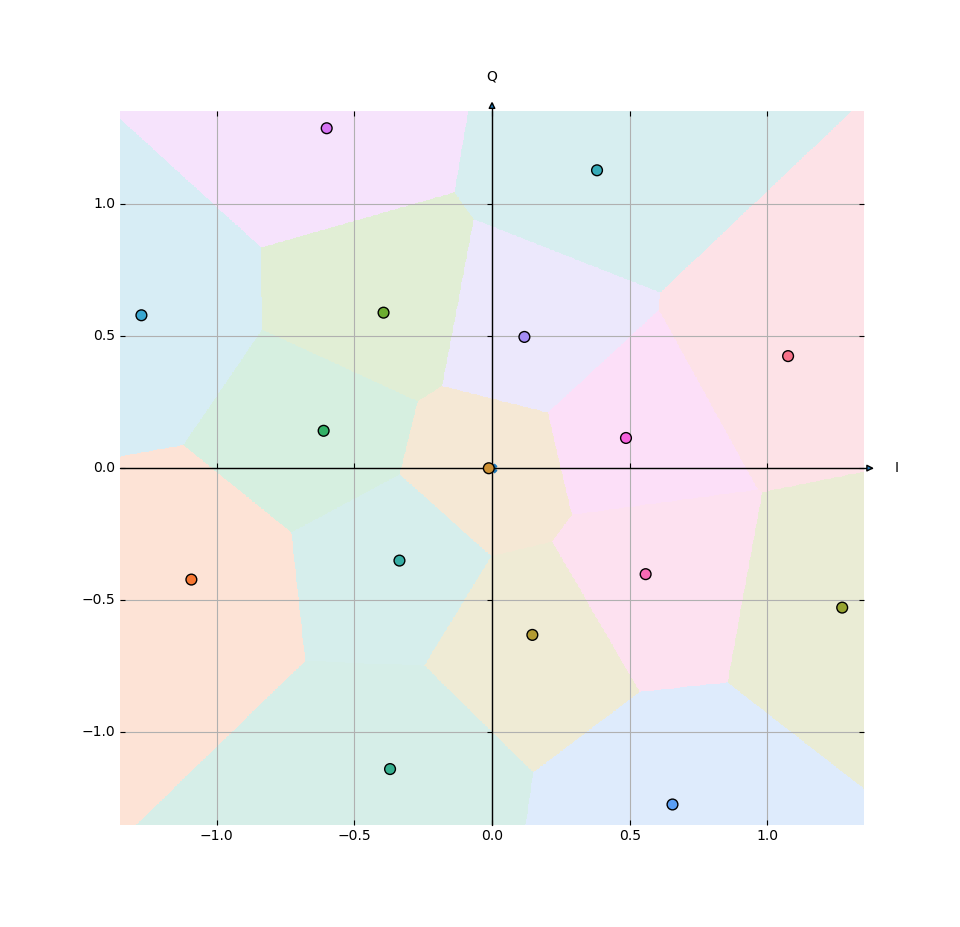
plot.py generates plots of trained models. It loads a trained model from output/constellation-order-X.pth where X is the order (can be changed at the top of the file). The constellation learned by the encoder is plotted as points and the decision regions learned by the decoder as colored areas around these points.
Experimentation
experiment.py runs experiments to find the best hyperparameters for each constellation order. Currently, the following parameters are tested:
order, the number of points in the constellation, is 4, 16 or 32.initial_learning_rate, the first learning rate used by the optimizer, is10^-2,10^-1or1.batch_size, the number of training examples in each batch, expressed as a multiple oforder, is 8 or 2048.first_layer, the size of the first hidden layer, ranges from 0 to the constellation’s order in steps of 4 (0 meaning that there is no hidden layer).last_layer, the size of the second hidden layer, ranges from 0 tofirst_layer(because the second layer is never larger than the first).
For a total of 378 different configurations. To enable parallelizing the experimentation, this set of configurations can be partitioned using two arguments, the first one describes the total number of parts to divide the set into and the second one which part number is to be tested.
Results of this experiment are available in results/experiment.csv.
